
Eric Wang
August 5, 2021
AndrewNG-DL基础
AndrewNG-Deep Learning 基础
1 Logistic Regression Model
1.1 Binary Classification
To learn a classifier that can input an image represented by the feature vector
x, and predict the corresponding labely.
Notation——n training examples: ($ n_x $为向量维数,$X$为$ n_x\times m $矩阵) $$ (x^{(1)},y^{(1)}),(x^{(2)},y^{(2)}), …, (x^{(m)},y^{(m)}),x\in R^{n_x}, y\in {0,1} $$
$$ X=[x^{(1)},x^{(2)},…,x^{(m)}], X\in R^{n\times m} $$
$$ Y=[y^{(1)},y^{(2)},…,y^{(m)}], Y\in R^{1\times m} $$
1.2 Logistic Regression
An algorithm for binary classification problems.
Given x, we want $\hat{y}=P(y=1|x)$
Way:
Parameters: $w\in R^{nx},b\in R$
Output: ($\sigma$为sigmoid函数,$\sigma(z)=\frac{1}{1+e^{-z}}$)
$$ \hat{y}=\sigma(w^Tx+b), (z = w^Tx+b) $$
1.3 Cost Function
we want $\hat{y(i)}\approx y(i)$
Loss(error) function: $L(\hat{y},y)=-(y·log\hat{y}+(1-y)log(1-\hat{y}))$
- $\hat{y(i)}$与$y(i)$越接近,$L(\hat{y},y)$越小
- If $y=1$: $L(\hat{y},y)=-log\hat{y}$
- If $y=0$: $L(\hat{y},y)=-log(1-\hat{y})$
It measures how well you’re doing on a single training example.
Cost function:$J(w,b)=\frac{1}{m}\sum_{i = 1}^{m}L(\hat{y}^{(i)},y^{(i)})$
It measures how well you’re doing on the entire training set.
1.4 Gradient Descent
An algorithm to learn the parameteres
wandbon your training set.
$$ w := w-\alpha\frac{\partial J(w,b)}{\partial w}, b:=b-\alpha\frac{\partial J(w,b)}{\partial b} $$
$\alpha$ is the learning rate.
Derivatives (导数)
Computation Graph
backward propagation
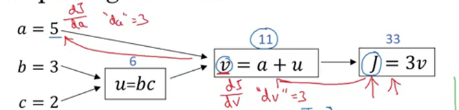
在代码中,可以用dv,da作为变量名。
$$ \frac{dJ}{dc}=\frac{dJ}{dv}\frac{dv}{du}\frac{du}{dc}=3\times1\times3=9 $$
Gradient Descent on 1 example
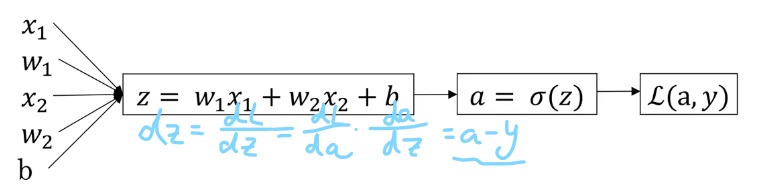 $$
w_1 := w_1-\alpha\frac{\partial dL}{\partial w},w_2 := w_2-\alpha\frac{\partial dL}{\partial w2},b := b-\alpha\frac{\partial dL}{\partial b}
$$
$$
w_1 := w_1-\alpha\frac{\partial dL}{\partial w},w_2 := w_2-\alpha\frac{\partial dL}{\partial w2},b := b-\alpha\frac{\partial dL}{\partial b}
$$
Gradient Descent on m examples
Neural network programming guideline: Whenever possible, avoid explicit for-loops.
Use vectorization.
Forward Propagation: $$ A=\sigma\left(w^{T} X+b\right)=\left(a^{(1)}, a^{(2)}, \ldots, a^{(m-1)}, a^{(m)}\right) $$
- Cost function:
$$ J=-\frac{1}{m} \sum_{i=1}^{m}\left(y^{(i)} \log \left(a^{(i)}\right)+\left(1-y^{(i)}\right) \log \left(1-a^{(i)}\right)\right) $$
Backward Propagation:
$$ \frac{\partial J}{\partial w}=\frac{1}{m} X(A-Y)^{T} $$
$$ \frac{\partial J}{\partial b}=\frac{1}{m} \sum_{i=1}^{m}\left(a^{(i)}-y^{(i)}\right) $$
Code of Optimizing procedure:
def propagate(w, b, X, Y):
    m = X.shape[1]

    # Forward propogation
    A = sigmoid(np.dot(w.T, X)+b);
    cost = -np.average(Y*np.log(A)+(1-Y)*np.log(1-A))

    #Backward propagation
    dw = np.dot(X, (A-Y).T)/m
    db = np.average(A-Y)

    cost = np.squeeze(np.array(cost))
    grads = {"dw": dw,
             "db": db}
    return grads, cost


def optimize(w, b, X, Y, num_iterations=100, learning_rate=0.009, print_cost=False):
    for i in range(num_iterations):
            grads, cost = propagate(w, b, X, Y)
            dw = grads["dw"]
            db = grads["db"]
            w = w - learning_rate*dw;
            b = b - learning_rate*db;
1.5 Python Skill
Broadcasting
A = np.array([1,2,3,4],
			[5,6,7,8],
			[9,10,11,12])
cal = A.sum(axis=0) # axis=0垂直方向求和,axis=1水平方向求和
percentage=A/cal.reshape(1,4) # broadcasting(1,4)->(3,4))
不要用rank=1(秩为1)的array,而要用5*1的矩阵
a = np.random.randn(5) # bad
a = np.random.randn(5,1) # good
assert(a.shape==(5,1))
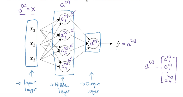
2 One hidden layer Neural Network
2.1 Neural Network Representation
One hidden layer NN also called a two layer NN (不算输入层)
2.2 Forward Propagation
On single training example:
$$ z^{[1]}=W^{[1]} x+b^{[1]}, a^{[1]}=\sigma(z^{[1]}) $$
$$ z^{[2]}=W^{[2]} a^{[1]}+b^{[2]}, a^{[2]}=\sigma(z^{[2]}) $$
vectorizing across multiple examples:
 $$
Z^{[1]} =W^{[1]} X+b^{[1]},A^{[1]}=g^{[1]}(Z^{[1]}),
$$
$$
Z^{[1]} =W^{[1]} X+b^{[1]},A^{[1]}=g^{[1]}(Z^{[1]}),
$$
$$ Z^{[2]} =W^{[2]} A^{[1]}+b^{[2]},A^{[2]}=g^{[2]}(Z^{[2]})=\sigma(Z^{[2]}) $$
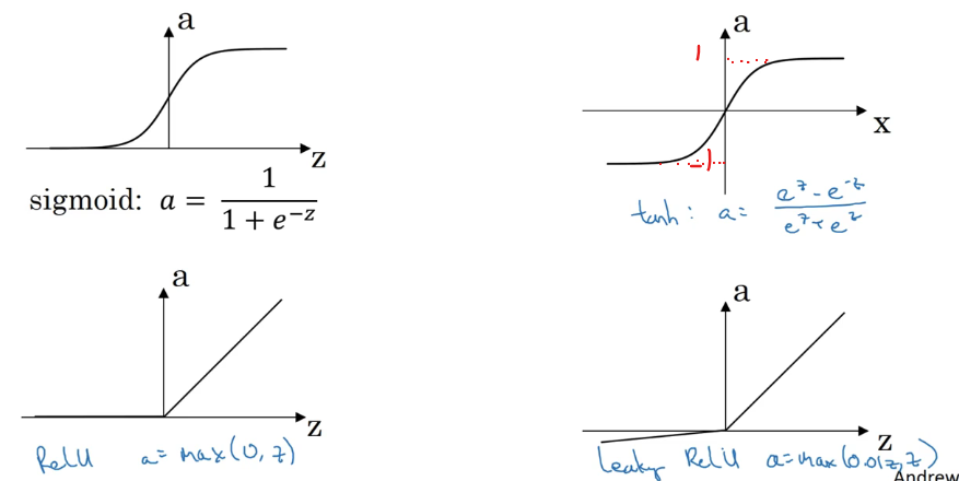
2.3 Activation functions
- tanh: $a=\frac{e^z-e^{-z}}{e^z+e^{-z}}$
tanh函数在绝大多数场景下比$\sigma$函数更适合用作激活函数;唯独在binary classification的输出层,$\sigma$函数更适合用作激活函数。
- Relu: a=max(0, z)
Relu函数可解决梯度消失的问题,优于tanh函数和$\sigma$函数。除了输出层,默认作为激活函数。
- Leaky Relu: a = max(0.01z, z)
2.4 Derivatives of Activation functions
- g(z)=$\sigma$(z): $g'(z)=a(1-a)$
- g(z)=tanh(z): $g'(z)=1-a^2$
- ReLU:
$$ g'(z)=\left\{ \begin{aligned} 0 & & z<0 \\ 1 & & z\geq0 \end{aligned} \right. $$
- Leaky ReLU:
$$ g'(z)=\left\{ \begin{aligned} 0.01 & & z<0 \\ 1 & & z\geq0 \end{aligned} \right. $$
2.5 Gradient descent for neural networks
backward propagation:
$$ dZ^{[2]}=A^{[2]}-Y $$
$$ dW^{[2]}=\frac{1}{m}dZ^{[2]}A^{[1]T} $$
$$ db^{[2]}=\frac{1}{m}np.sum(dZ^{[2]},axis=1,keepdim=True) $$
$$ d Z^{[1]}=W^{[2] T} d Z^{[2]} * g^{[1]^{\prime}}\left(\mathrm{Z}^{[1]}\right) $$
$$ d W^{[1]}=\frac{1}{m} d Z^{[1]} X^{T} $$
$$ d b^{[1]}=\frac{1}{m} np.sum(d Z^{[1]}, axis=1, keepdims=True) $$
- keepdim=True: 用于防止输出$(n^{[2]},)$,而是输出$(n^{[2]},1)$
2.6 Random Initialization
在Neural network中,w不能初始化为全0。
$$ w^{[1]}=np.random.randn((2,2))*0.01 $$
$$ b^{[2]}=np.zero((2,1)) $$
$$ w^{[1]}=np.random.randn((1,2))*0.01 $$
$$ b^{[2]}=0 $$
3 Deep Neural Network
- layers: L = 4
- ouput: $\hat{y}=a^{[L]}$
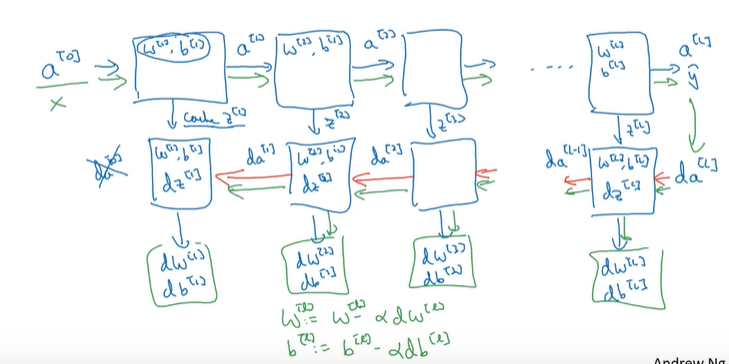
3.1 Forward Propagation
for l=1…4: $$ Z^{[l]}=W^{[l]}A^{[l-1]}+b^{[l]} $$
$$ A^{[Ll}=g^{[l]}(Z^{[l]}) $$
3.2 Backward Propagation
- Input $da^{[l]}$
- Output $da^{[l-1},dW^{[l]},db^{[l]}$
$$ dZ^{[l]}=dA^{[l]}*{g^{[l]}}'(Z^{[l]}) $$
$$ dW^{[l]}=\frac{1}{m}dZ^{[l]}·A^{[l-1]T} $$
$$ db^{[l]}=\frac{1}{m}np.sum(dZ^{[l]},AXIS=1, keepdims=True) $$
$$ dA^{[l-1]}=W^{[l]T}dZ^{[l]} $$
3.3 Matrix dimensions
- $W^{[l]},dW^{[l]}:(n^{[l]},n^{[l-1]})$
- $b^{[l]},db^{[l]}:(n^{[l]},1)$
- $z^{[l]},a^{[l]}:(n^{[l]},1)$
- $Z^{[l]},A^{[l]},dZ^{[l]},dA^{[l]}:(n^{[l]},m)$
3.4 Working procedure
3.5 Parameters & Hyperparameters
Hyperparameters control the parameters.
Paramerters:
- $W^{[a]},b^{[a]}$
Hyperparematers:
- learning rate $\alpha$
- iterations
- hidden layers L
- ……